Turing Machine
matsuda@symbolics.jp
(ref. "Computer Science with Mathematica", Roman E. Maeder)
Computable Functions
![]()
we can define addition and multiplication over natural numbers.
Primitive Recursive Functions
1. the constant 0
2. the successor function
3. the projection function ![]()
![]()
4. the composition of primitive recursive functions.
Let ![]() be primitive recursive, n≥ 0
be primitive recursive, n≥ 0
![]()
5. Let f and g be primitive recursive, n≥ 0, and
![]()
Then, h is a P.R.F.
the addition ![]() ) is a primitive recursive function:
) is a primitive recursive function:

conditional statements as primitive recursive functions
![]() for k=0,
for k=0, ![]() for k>0
for k>0
![]()
functions defined with bounded iteration are primitive recursive functions
Mathematica Do loop is it. But
![]()
Mathematica While loop is not. (not be promised with finite iterations)
Partial Recursive Functions
be not defined on total N. for example, the square root, which define only on 0,1,4,9,…
so add a new scheme to the primitive recursive functions
6. (μ scheme) Let f and g be primitive recursive
![]()
is a partial recursive function.
![]() is the least k with
is the least k with ![]() , if one exists
, if one exists
undefined otherwise.
ex. the squre root function Let
![]()
![]() is zero if and only if
is zero if and only if ![]() . now define the square root function w(m):
. now define the square root function w(m):
![]() .
.
the μ schema formalize the While loop.
![]()
if m is not a square, the loop will not terminate! “Undefined” usually means for functions given by programs that the program does not terminate.
Ackermann Function
All primitive recursive function are total. Partial recursive function may be - but need not be - total. The class of recursive functions is the class of all partial recursive functions that are total.
There exists a total function that is not primitive recursive, such that is the Ackermann function.

It can be shown that primitive recursive functions cannot grow too fast. If A(x,y) were primitive recursive, then f(n)=A(n,n) would also be primitive recursive. This is impossible because ![]() grows faster than
grows faster than ![]() for
for ![]() . There should be a
. There should be a ![]() , such that
, such that ![]() .
.
![]()
![]()
![]()
![]()
![]()
![]()
![]()
![]()
![]()
![]()
![]()
Recursive Functions are Computable
We have to convince ourselves that the schema of primitive recursive, and the μ schema can be programmed with Mathematica or TM.
![]()
![]()
![]()
Models of Computation
Which functions can be computed at all? Abstract machine. One candidate is the Turing machine. The simplicity of the Turing machine allows us to prove that every function computable on it is partial recursive. The computable functions are exactly the partial recursive functions.
Equivalence of Machine Models
An important tool for proving two models equivalent is simulation.
The program Mathematica is nothing but an interpreter of Mathematica’s programming language on a certain computer.
ex. An interpreter of Turing machines in Mathematica
The Halting Problem
Is there a program H that can find out whether another program P with input E will halt in finite time? A total function H(P,E) returns 0 if P halts with input E, and 1 otherwise.
Contradiction! Define
![]()
If H were computable, G would be, too. Look at G(G): The execution of programG with input G terminates if and only if H(G,G)>0, that is, if program G with input G does not halt!
Therefore, the halting problem is undecidable, that is, there is no program that can decide whether any program halts on any given input.
Background Idea of Turing Machine
ref. http://en.wikipedia.org/wiki/Turing_machine
Automatic Machine (Alan Turing 1936)
Hypothetical device representing a computing machine
“Intelligent Machinery” (1945 Essay)
Turing Machine consists of the following device and the functions
(1)an infinite tape
(2)a head which read/writes a symbol on the tape and can move one position
(3)a state register which memorize the current position of the head on the tape
(4)a rule table(program) which decides the next action to the tape head
The original idea comes from the following fundamental question:
[Hilbert’s tenth question of 1900]
10. Determination of the solvability of a Diophantine equation. Given a Diophantine equation with any number of unknown quantities and with rational integral coefficients: To devise a process according to which it can be determined in a finite number of operations whether the equation is solvable in rational integers. The Entscheidungsproblem [decision problem for first- order logic] is solved when we know a procedure that allows for any given logical expression to decide by finitely many operations its validity or satisfiability ... The Entscheidungsproblem must be considered the main problem of mathematical logic.
—quoted, with this translation and the original German, in Dershowitz and Gurevich, 2008
Allan Turing proofed this question with a negative answer and invented a Turing Machine as a secondary effect.
“The theory of computation has traditionally been studied almost entirely in the abstract, as a topic in pure mathematics. This is to miss the point of it. Computers are physical objects, and computations are physical processes. What computers can or cannot compute is determined by the laws of physics alone, and not by pure mathematics”
– David Deutsch (one of top runners in quantum computing )
Q.What is computation?
A. Proof not with inductive method but with constructive method (Turing Machine) by using the following rough(not in Turing Machine but here) computing parts:
zero
successor
while
compose
...
Lego Turing Machine
Automatic Computing Engine (ACE) designed by Alan Turing(1946), finished on 1954.
The Machine Model
It writes a symbol into the cell under head, overwriting the symbol present. The new symbol may be the same as the old one, in which case the contents of the cell are not changed.
It moves the head one cell to the right or left, or it stays where it is. We denote this action by l, r, and s.
The machine enters a new state.
Preparing a Tape
Assuming an infinite tape. The function tape creates a tape which contents is given by list and which head is specified by offset. The symbol indicates a blank.
![]()
ref. Array[t,6]-->{tape[...][1], tape[...][2],tape[...][3]....}
![]()
![]()
![]()
![]()
updating the tape
ref. /: TagSetDelayed define ‘module’ operation
![]()
![]()
![]()
stack example
![]()
![]()
![]()
![]()
![]()
![]()
![]()
finding a non-blank position
![]()
![]()
![]()
![]()
![]()
![]()
![]()
![]()
![]()
![]()
new tape
For example newTape[1,b] supposes p0 is 1, so the offset of this tape will be 0(p0-1).
![]()
![]()
![]()
Defining a Turing machine with configuration and instruction
Plot Configuration
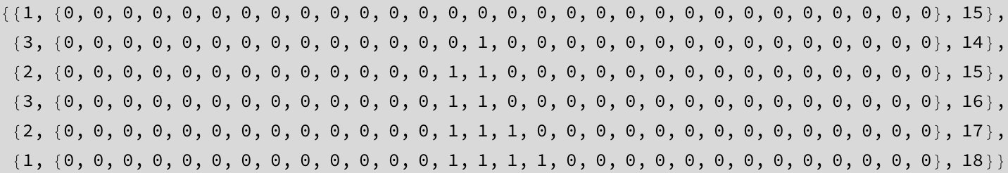
initial configuration
The left most 1 of config indicates the state number and the right most 1 indicates the position of the tape.
![]()
![]()
![]()
Instructions

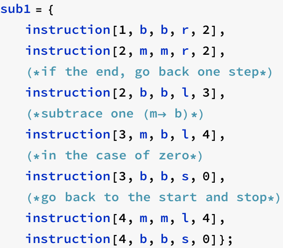
Example. Instruction set for subtracting one from the current value. In the initial step, the state is 1 and the current value is b then moves the head to the right and changes the status to 2 (the first instruction).
| {1,b}→{b,r,2} |
| {2,m}→{m,r,2} |
| {2,b}→{b,l,3} |
| {3,m}→{b,l,4} |
| {3,b}→{b,s,0} |
| {4,m}→{m,l,4} |
| {4,b}→{b,s,0} |
updating a configuration
3 - 1
computes 3 - 1. Three marks will be decreased two ones.
![]()
![]()
![]()
![]()
![]()
![]()
![]()
| config[1,< b m m m b b ...>,1] |
| config[2,< b m m m b b ...>,2] |
| config[2,< b m m m b b ...>,3] |
| config[2,< b m m m b b ...>,4] |
| config[2,< b m m m b b ...>,5] |
| config[3,< b m m m b b ...>,4] |
| config[4,< b m m b b b ...>,3] |
| config[4,< b m m b b b ...>,2] |
| config[4,< b m m b b b ...>,1] |
| config[0,< b m m b b b ...>,1] |
| config[0,< b m m b b b ...>,1] |
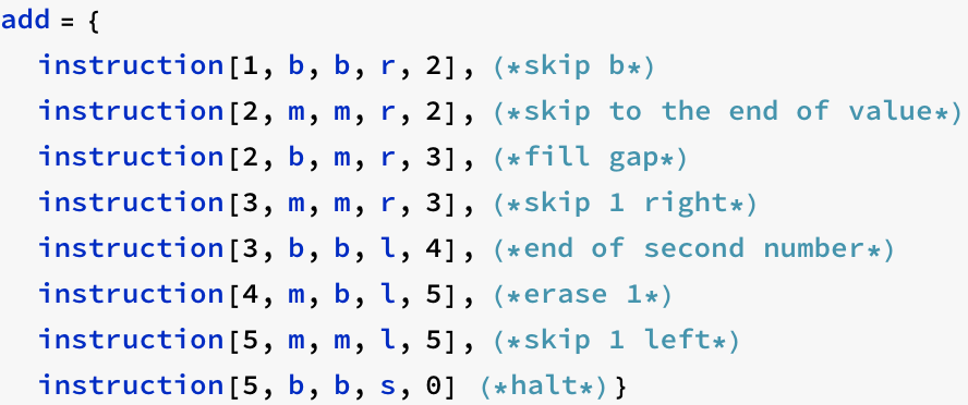
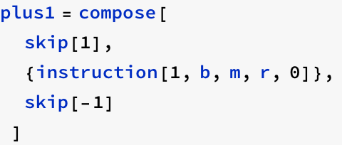
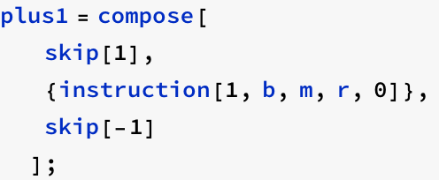
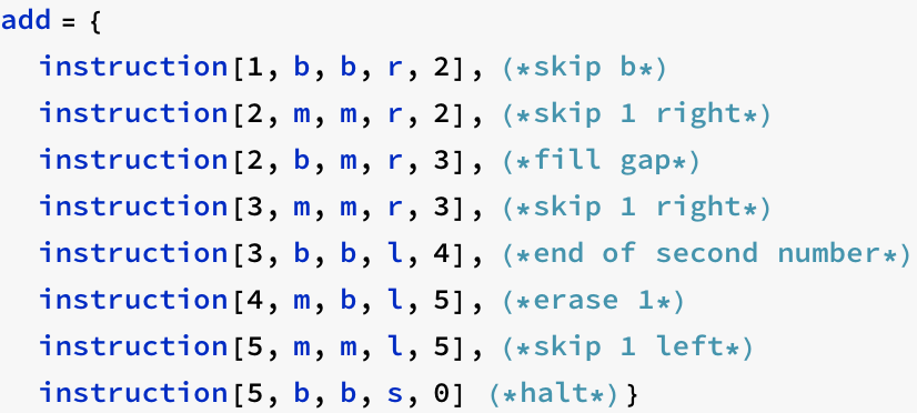
add
![]()
![]()
![]()
![]()
![]()
defining a run
1+3
![]()
a sub b, supposing a > b
3 - 2
![]()
Assembler for Turing Machine
Following controls are available: right, while, skip[n], skip[-n], shifleft[n], eat1[n], copy[n,m]
How to compose number of instructions
Should relocate for sates. like allocating absolute address for relative address in compiler.
First example is right. This command consists of two instructions for moving the head one step to the right according to the current values b and m. Note the target state should be 0 because correct value will be assigned when command composition.
![]()

right; right;
in the first right, the offset is 0, transition is 1 to 2. in the second right, the offset is 1 and the transition is 0.
![]()
![]()
compose
automatically to compose several commands like compose[right, right].
ref. tutorial/FlatAndOrderlessFunctions
![]()

![]()
![]()
![]()
![]()
![]()
![]()
![]()
![]()
while
![]()
![]()

![]()
other commands

zero
![]()
![]()
![]()
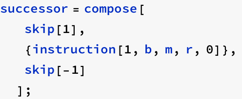
successor
![]()
![]()

Recursive Functions Are Turing Computable
We want to show that these functions can be computed on Turing machine.
The following requirements for the six construction principles for partial recursive functions.
[calling convention]
The natural number n is represented by n consecutive marks.
Arguments of a function are separated by exactly one blank.
The tape to the right of the argument is empty.
The computation starts in state 1 with the head on the blank immediately before the first argument.
The machine does not use the tape to the left of the initial cell.
At the end of a computation, the head is again on the initial cell with the result following on the right.
The Basic Functions
![]()
![]()
![]()
Projections
The projection ![]() returns argument
returns argument ![]() .
.

![]()

Composition
The macro comp[![]() ] generates the program for a function h, with
] generates the program for a function h, with
Primitive Recursion

Turing Machine, Mathematica version
Instructions

while

sub1
compose
other commands
![]()
The Basic Functions
![]()
![]()

![]()
![]()
Projections
The projection ![]() returns argument
returns argument ![]() .
.
Composition
![]()
provided that ![]() are programs for the corressponding functions. First, we must evaluate the function
are programs for the corressponding functions. First, we must evaluate the function ![]() with arguments
with arguments ![]() , and then apply the function f to the p resuls. Because we need the original arguments several times, we copy them to the end of the tape and run the program for
, and then apply the function f to the p resuls. Because we need the original arguments several times, we copy them to the end of the tape and run the program for ![]() on this copy.
on this copy.
Figure 12.4-1 shows that idea. Line a) shows the initial configuration with n arguments on the tape. We copy them to the end (line b). Now we can run the program for ![]() ; it leaves a result
; it leaves a result ![]() , as shown in line c. Accoridng to our calling convention, the program does not use the arguments again the tape to the left of the initial posiiton, a property that is important here.Now, we copy the arguments again, ready to run
, as shown in line c. Accoridng to our calling convention, the program does not use the arguments again the tape to the left of the initial posiiton, a property that is important here.Now, we copy the arguments again, ready to run ![]() (line d). Line e shows the tape after all programs
(line d). Line e shows the tape after all programs ![]() were run. We can now delete the original arguments and run f, as shown in line f. The last line shows the final result.
were run. We can now delete the original arguments and run f, as shown in line f. The last line shows the final result.
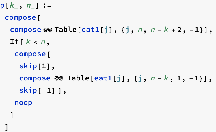
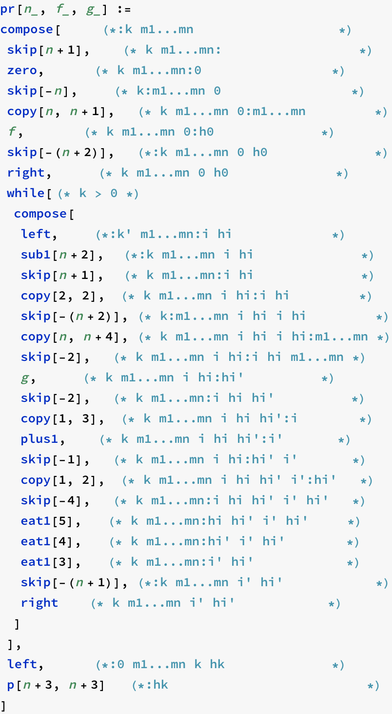
Primitive Recursion
The macro pr[n,f,g] generates the program for a function h with
provides that f and g are programs for the respective functions. The Turing machine does not offer recursion, so we have to turn it into iteration.
First, we compute ![]() =h[
=h[![]() ], by calling
], by calling ![]() . In the loop, we repeatedly compute
. In the loop, we repeatedly compute ![]() for i=0,1,...
for i=0,1,...
After each iteration, we decrement k until we reach k=0. The details are rather awkward. The comments in the program in the next listing show the tape in an abbreviated way. The head position is marked by :, unless the head happens to be inside an argument.
![]()
![]()
![]()
![]()
![]()
![]()
![]()
![]()
![]()
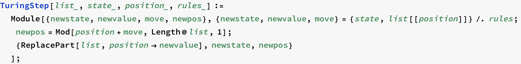
Mathematica TuringMachine function
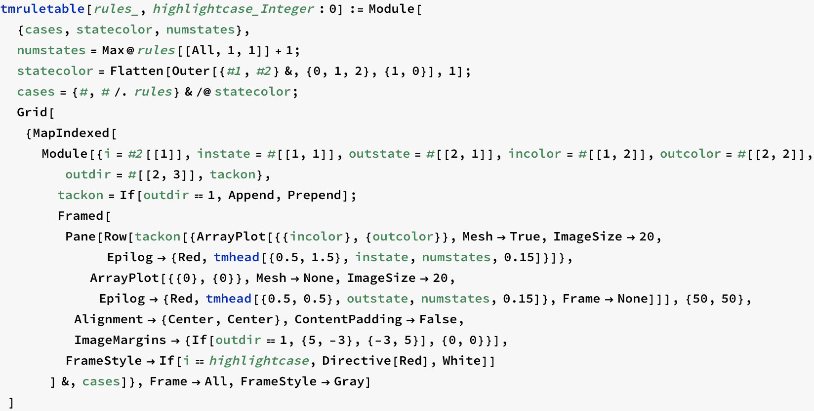
TM explanation
“Hunting for Turing Machines at the Wolfram Science Summer School”
ref. http://blog.wolfram.com/2012/12/20/hunting-for-turing-machines-at-the-wolfram-science-summer-school/
The rules of a Turing machines are actually super simple. There’s a row of cells called the tape:
![]()
![]()
Then there's a head that sits on the tape like so:
the state is {0,1,2} and the color is {1,0}. The state is the step index of the head transition and the color is the value on the tape.
The following example describes a group of state-color combination: {state0, color1}, {state0, color0},{state1, color1}, {state1, color0}, {state2, color1}, {state2, color0}.
![]()
![]()
![]()
![]()
![]()
![]()
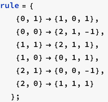
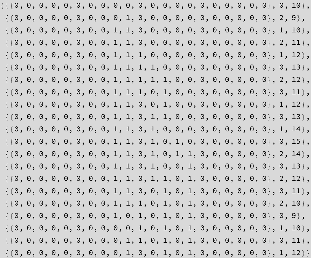
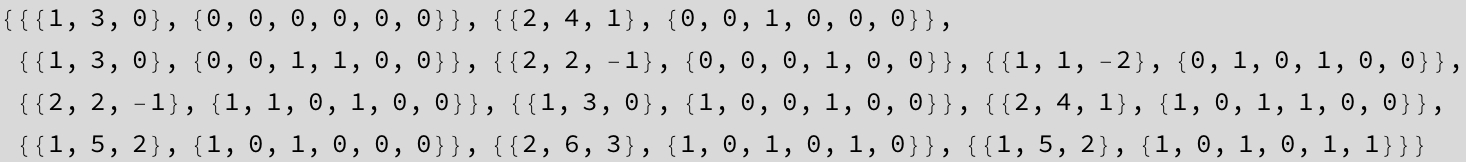
rule: {state, color} →{new-state, new-color, offset}
![]()
![]()
![]()
![]()
![]()
![]()
state=0 color=0 position=10 → state=2 Position-1
state=2 color=0 position=9 → state=1 Position+1
state=1 color=1 position=10 → state=2 Position+1
state=2 color=0 position=11 → state=1 Position+1
....
![]()
![]()

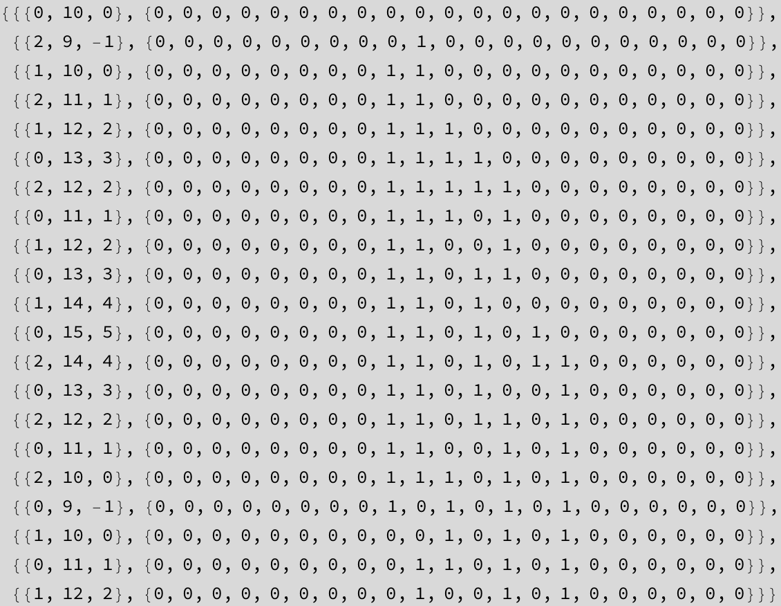
the sequence of the applied rules
![]()
![]()
![]()
![]()
![]()

![]()

![]()
The head can point in different directions to show what state it’s in. Let’s say there are just three possible states, so the head can point in three different directions:

In addition, each cell on the tape has a color. In the simplest case there are just two possible colors, black or white (binary):
![]()
![]()
So for each of the three head states, there are two possible cell colors, giving six different situations:

| white | |||
| black | |||
| state 1 | state 2 | state 3 |
The rule table tells the Turing machine what to do in each situation:
![]()
 |
 |
 |
 |
 |
 |
You can see how it works: the cell under the head changes color, then the head moves left or right and updates its state.
So let’s say the head is in state 1 on a blank tape:

![]()
We look up the case in the rule table where the head is on a white cell in state 1:
![]()
 |
 |
 |
 |
 |
 |
The rule says the cell under the head changes to black; the head moves left, and goes into state 3:


Notice we are showing the updated tape right below the old one. That way we can see where the head was on the previous step and where it is currently.
Now the head is in state 3 on a white cell, so we look that case up:
![]()
 |
 |
 |
 |
 |
 |
The rule says the cell changes to black; the head moves right, and goes into state 2:

Now the head is in state 2 and this time it’s on a black cell:
![]()
 |
 |
 |
 |
 |
 |
The rule says the cell stays black; the head moves right, and goes into state 3:


Getting the hang of it? Pretty simple, right? Here’s what the Turing machine evolution looks like after 20 steps:

TMStep (NKS version chap.3)
![]()
![]()
Numbering Scheme
ref. NKS page 888
無限の空テープの2状態,2色のマシン2506:
![]()
![]()


![]()
![]()
![]()
![]()
![]()
![]()
![]()
![]()
![]()
![]()
![]()
![]()
![]()

![]()
状態の情報をテープの表現に「注入」する:
![]()
![]()
頭部の位置を赤い正方形で示す:
![]()
Rule number of a machine whose instruction table is given:
ref. http://www.physinfo.org/annexes/suites/CompressionMTS.html
![]()
![]()
![]()
![]()
![]()
![]()
![]()
Assembler
テープに対する操作命令の集まりからマクロ命令(通常は,より人間にわかりやすい名前が付く)を作ります.本来ならば,このマクロ命令からテープ操作の命令instructionへの変換が必要となりますが,マクロ命令自身が関数となっているため,定義した時点でinstructionの列となります.命令の合成において唯一必要なことは,
(1)個々のinstructionに対し,offset値によって現在の状態番号を変える.
(2)終了状態に対しては0が,そうでない場合は,現在の状態,次の状態共にoffset値で変更する.
の2つです.
たとえば,テープを右に移動するというマクロ命令 right を考えると,right は次の2つのテープ命令からなります.
![]()
![]()
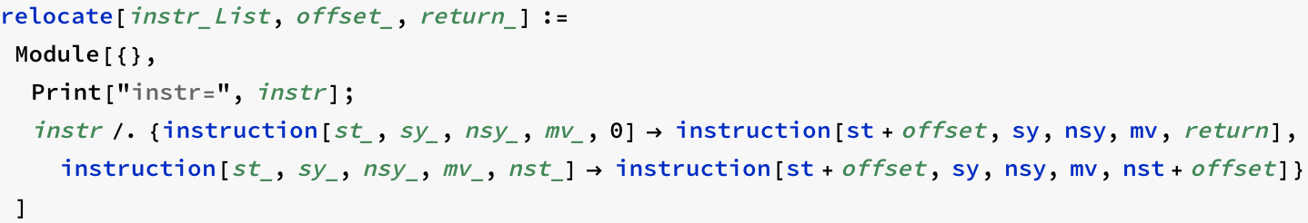
このマクロ命令 right を使い,連続して右に移動するというプログラム right; right; をテープ命令に変換することを考えます.この時,状態番号に関する変更が必要となってきます.それを実現する関数が次の relocate です.ここで,instrには複数の命令が来ることに注意してください.

right; right プログラムの右側の right に対する状態の変更を行います.状態番号を1増やし,終了状態0とします.
![]()
![]()
一方,左側right に関しては,状態番号の変更はなく,次の状態returnのみを2に変更します.
![]()
![]()
最後に,この2つの命令群をあわせます.
![]()
![]()
1.マクロ命令の合成
2個以上のマクロ命令からなるプログラムをテープ命令に変換することを考えます.
上記関数で,instr2 には2個以上の命令のリストが束縛され,これをどう処理するかが問題となります.SetAttributesで2つの属性をセットすることで,うまく処理されますが,どういう動きになるかを見るために,relocateを以下のように再定義し,instrに渡される値をプリントしてみることにします.
この例の場合は,特に変わったところはありません.
![]()
![]()
![]()
![]()
ここでは,マクロ命令は3つしかないのに,relocateは4回呼ばれています.なお,このプログラムは,テープを3回読み,そこで停止する命令からなります.
![]()
![]()
![]()
![]()
![]()
![]()
composeに対し,上記のような属性をセットした時,2個以上の値をセットされた変数を使う関数があるとき,
![]()
![]()
![]()
![]()
のような計算を行います.次の例も理解してみてください.
![]()
![]()
![]()
![]()
![]()
![]()
![]()
![]()
![]()

1.1 While
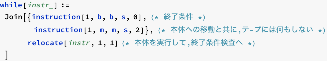
状態2においてブランクを読めば停止.さもなければ,状態2と3を交互に行き来する.

![]()
![]()

2. 他のマクロ
skip[n]
skip[-n]
shiftleft[n]
eat1[n]
copy[n,m]

2.1基本関数
![]()
![]()
![]()
![]()

![]()
![]()
![]()
Example
![]()
![]()
![]()
TuringMachine--テープ--
左右に無限に延びるテープを仮定.関数 tape は,指定した記号の列からなるテープを表す.b はブランク記号.offsetは,テープ読み取りヘッドの位置.
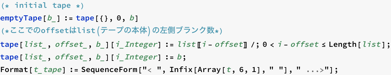
初期テープ
![]()
空のテープ.初期テープ.
テープの定義
![]()
![]()
listを要素に持つテープ.ただし,offsetが0でない時,listの先頭にヘッドがあり,それより右に,offset分のブランクbが入る.次の例参考.
![]()
![]()
![]()
![]()
![]()
![]()
![]()
Formatを定義することで,tapeをヘッドに持つデータを出力する時,常にここで指定した形式で表示する.テープ中の幅6の部分を表示.上記例で,{b,m,m}でオフセットが1なので,テープの左側にブランクが1つ,右側に2個のブランクが入る.
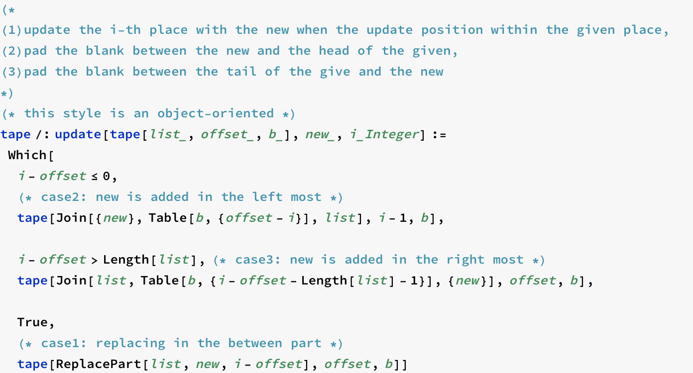
テープの書き換え
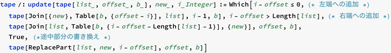
![]()
tape /: update[tape[....]] では,tape:/の部分はなくても良いが,tape:/以下をtapeに関する手続き(メソッド)という風にobject-orientedなプログラミングスタイルになっている.
![]()
![]()
![]()
![]()
![]()
![]()
テープt2の8番目は見えていないが,その左にブランクが入り,8番目にマークmが入っていることが t2[8] の結果でわかる.
非ブランク位置
左端での非ブランク位置を low, 右端での非ブランク位置を high で表す.
![]()
![]()
![]()
![]()
![]()
![]()
テープの作成
![]()
p0のデフォルト値は1 .したがって,newTape[l, b]の時,tapeへのオフセット p0-1 は0.
TuringMachine--配置と命令--
チューリングマシンを配置(configuration)と,配置を書き換える命令(instruction)によって定義する.
配置: config[ state, tape, head]
命令: instruction[state, symbol, newsymbol, move, newstate]
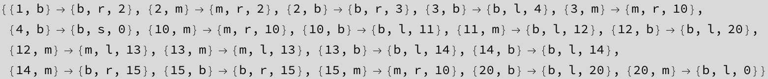
{state, symbol} → {newsymbol, move, newstate}
初期配置
![]()
![]()
![]()
config の左側の1 は出発状態を表す.状態は順次番号付けされる.右端の 1はテープヘッドの位置.この例だと,右端のブランク b の位置にある.なお,このモデルでは,テープの最初にブランクが一つ,複数のマーク群を作る時は,ブランクを一つとする.
命令
| {1,b}→{b,r,2} |
| {2,m}→{m,r,2} |
| {2,b}→{b,l,3} |
| {3,m}→{b,l,4} |
| {3,b}→{b,s,0} |
| {4,m}→{m,l,4} |
| {4,b}→{b,s,0} |
[命令の読み方] 状態に1にあって,テープヘッドが b を読んだら,テープはそのままヘッドを右に移動し,状態を2に変更.状態2にあって,テープヘッドが m を読んだら,テープはそのままでヘッドを右に移動し,状態は2のまま.つまり,この2つ目のルールはテープ上に m がある間,読み飛ばすこと表している.
配置の書き換え
![]()
![]()
![]()
| config[1,< b m m m b b ...>,1] |
| config[2,< b m m m b b ...>,2] |
| config[2,< b m m m b b ...>,3] |
| config[2,< b m m m b b ...>,4] |
| config[2,< b m m m b b ...>,5] |
| config[3,< b m m m b b ...>,4] |
| config[4,< b m m b b b ...>,3] |
| config[4,< b m m b b b ...>,2] |
| config[4,< b m m b b b ...>,1] |
| config[0,< b m m b b b ...>,1] |
いま,m の個数で数を表すとすると,命令 sub1 は3-1を計算したことになる.最後の配置で状態は0なので計算は終了.
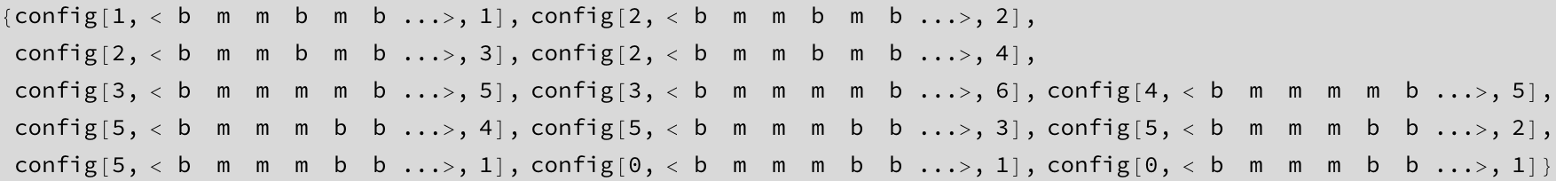
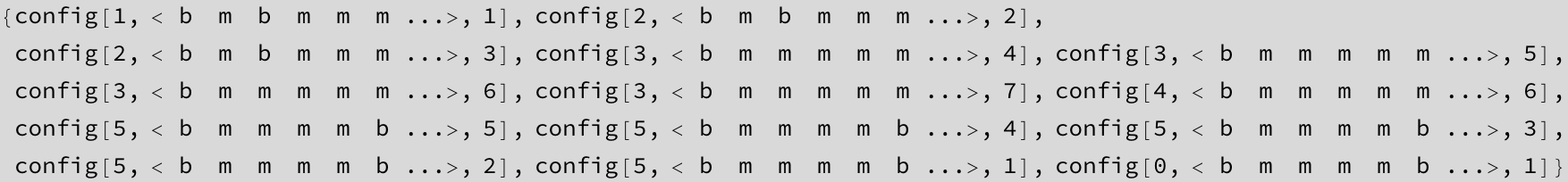
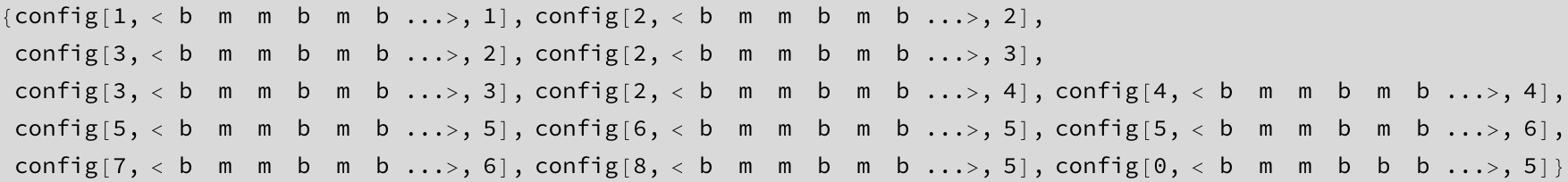
例題
![]()
![]()
![]()
![]()
| config[1,< b m m b m b ...>,1] |
| config[2,< b m m b m b ...>,2] |
| config[2,< b m m b m b ...>,3] |
| config[2,< b m m b m b ...>,4] |
| config[3,< b m m m m b ...>,5] |
| config[3,< b m m m m b ...>,6] |
| config[4,< b m m m m b ...>,5] |
| config[5,< b m m m b b ...>,4] |
| config[5,< b m m m b b ...>,3] |
| config[5,< b m m m b b ...>,2] |
| config[5,< b m m m b b ...>,1] |
| config[0,< b m m m b b ...>,1] |
| config[0,< b m m m b b ...>,1] |
| config[0,< b m m m b b ...>,1] |
| config[0,< b m m m b b ...>,1] |
| config[0,< b m m m b b ...>,1] |
| config[0,< b m m m b b ...>,1] |
| config[0,< b m m m b b ...>,1] |
| config[0,< b m m m b b ...>,1] |
| config[0,< b m m m b b ...>,1] |
| config[0,< b m m m b b ...>,1] |
![]()
| config[1,< b m m b m b ...>,1] |
| config[2,< b m m b m b ...>,2] |
| config[2,< b m m b m b ...>,3] |
| config[2,< b m m b m b ...>,4] |
| config[3,< b m m m m b ...>,5] |
| config[3,< b m m m m b ...>,6] |
| config[4,< b m m m m b ...>,5] |
| config[5,< b m m m b b ...>,4] |
| config[5,< b m m m b b ...>,3] |
| config[5,< b m m m b b ...>,2] |
| config[5,< b m m m b b ...>,1] |
| config[0,< b m m m b b ...>,1] |
| config[0,< b m m m b b ...>,1] |

![]()
![]()
![]()

TuringMachine--配置と命令--
(課題解答)
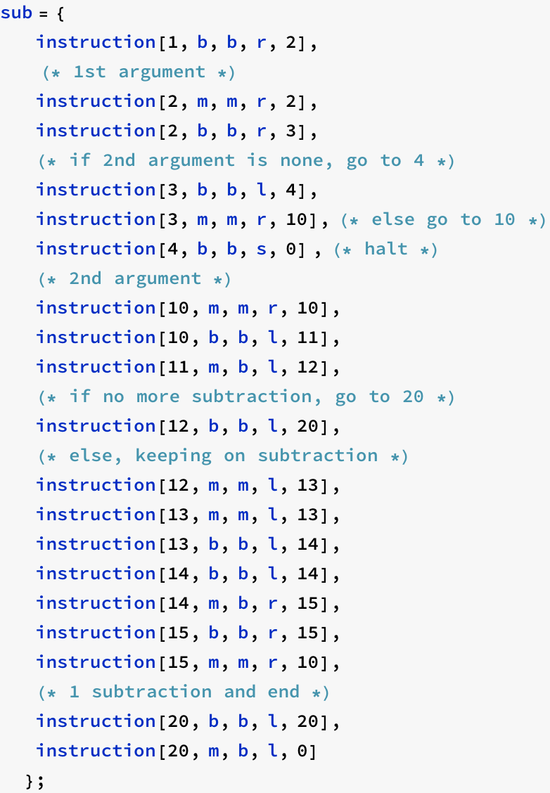
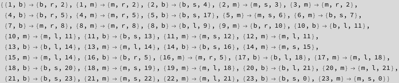
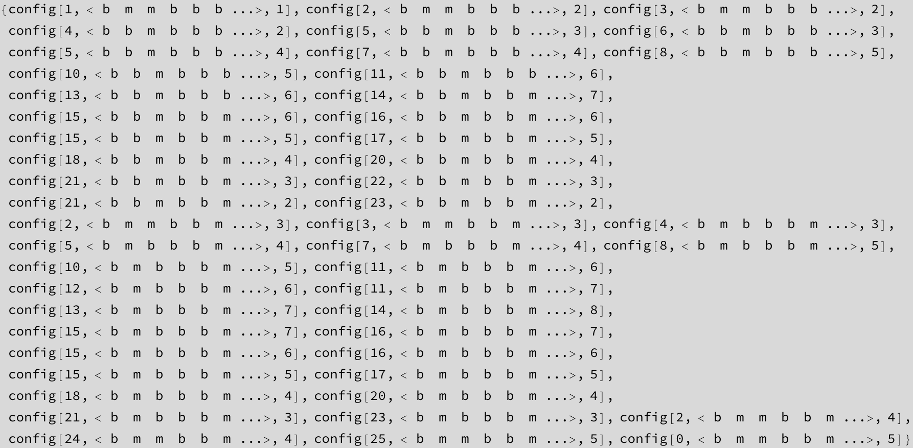
【課題】引き算subを定義しなさい.ただし,第1引数は第2引数より大きいものと仮定します.
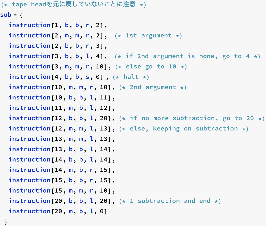
![]()
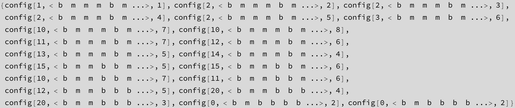
| config[1,< b m m m b m ...>,1] |
| config[2,< b m m m b m ...>,2] |
| config[2,< b m m m b m ...>,3] |
| config[2,< b m m m b m ...>,4] |
| config[2,< b m m m b m ...>,5] |
| config[3,< b m m m b m ...>,6] |
| config[10,< b m m m b m ...>,7] |
| config[10,< b m m m b m ...>,8] |
| config[11,< b m m m b m ...>,7] |
| config[12,< b m m m b m ...>,6] |
| config[13,< b m m m b m ...>,5] |
| config[14,< b m m m b m ...>,4] |
| config[15,< b m m b b m ...>,5] |
| config[15,< b m m b b m ...>,6] |
| config[10,< b m m b b m ...>,7] |
| config[11,< b m m b b m ...>,6] |
| config[12,< b m m b b b ...>,5] |
| config[20,< b m m b b b ...>,4] |
| config[20,< b m m b b b ...>,3] |
| config[0,< b m b b b b ...>,2] |
| config[0,< b m b b b b ...>,2] |
Assembler
Intelチップ上の命令をコンピュータの機械語(machine language)と見ると,Turingテープ上の操作はTuringMachineというコンピュータの機械語命令の集まりとみることができる.通常,機械語に対してはより人間に分かりやすい命令セットしてAssembly 言語が考えられており,プログラミング言語,たとえば,C言語などはcompilerによって一旦,Assembly言語に変換されるのが普通である.
そこで,ここでは,TuringMachineを前提にそのAssemblerを設計してみることにする.そのためには,まず,Assembly言語の設計が必要となる.主なものを以下に挙げる:
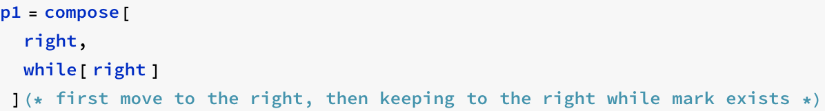
right
while
skip[n]
skip[-n]
shiftleft[n]
eat1[n]
copy[n,m]
これらの命令(マクロ)をTuringMachine上の命令(instruction, TM)を使って定義する.
なお,複数のinstructionをつなぎあわせるためには,
(1)個々のinstructionに対し,offset値によって現在の状態番号を変える.
(2)終了状態に対しては0が,そうでない場合は,現在の状態,次の状態共にoffset値で変更する.
の2つの考慮が必要となる.
たとえば,テープを右に移動するという命令 right を考えると,right は次の2つのTM命令からなる.ここで,どちらの場合も,遷移状態番号が0になっていることに注意.
![]()
![]()
![]()
この命令 right を使い,連続して右に移動するというプログラム
right; right;
をTM命令に変換することを考える.この時,状態番号に関する付け替えが生じる(通常,コンパイラやアッセンブラで複数の命令に対し,番地の再計算を行うのと同じこと).
遷移先が終了の場合は,最初の状態にのみoffsetを加えればよい.そうでない場合は,遷移先状態にも加える必要がある.

左側の right はオフセット0で,状態1から2へ遷移する.これを次のように定義する.
![]()
![]()
次に,右側の right に対しては,次の状態(2)から始めるためにオフセットを1にし,最終状態を0としてる.
![]()
![]()
最後に,この2つの命令群をあわせる.
![]()
![]()
1.マクロ命令の合成
上で,手動で合成したものを自動で合成したい.たとえば,
Compose[right, right]
のように.
![]()
![]()
![]()
しかし,この compose という関数は次のように3つ以上の命令を合成しようとすると失敗する.
![]()
![]()
そこで,n個の命令を合成できるよう関数composeに以下のような属性を与える.(詳細は省略)
![]()
![]()
![]()
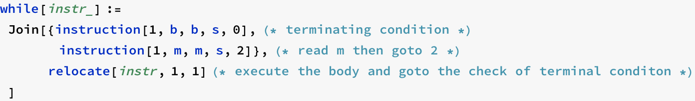
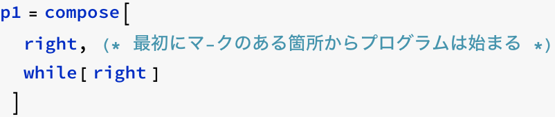
1.1 While

![]()
状態2においてブランクを読めば停止.さもなければ,状態2と3を交互に行き来する.
![]()
![]()

2. 他のマクロ
skip[n]
skip[-n]
shiftleft[n]
eat1[n]
copy[n,m]

![]()
|
2.1基本関数
![]()
![]()
![]()

![]()
Assembler(問題解答)
![]()

![]()
![]()